Track system
Pitch Track
The pitch track of the COMSAR framework extracts pitch from a soundfile, accumulates pitches into an octave, detects notes, vibrato, slurs, or melisma, determines most likely tonal systems, extracts the melody, and calculates n-gram histograms.
The pitch track instance should contain the frame size and hop ratio. In the example notebook 100 pitches per second are analyzed (see jupyter example notebook COMSAR_Melody_Example.jpynb)
Melody
An example of a Lisu solo flute piece (ESRA, vimeo) for pitch and melody extraction is shown in the figure below.
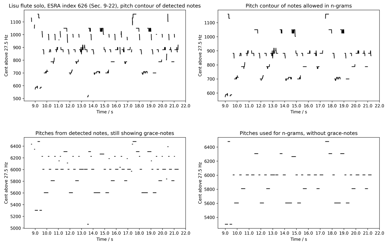
Example of pitch and melody extraction using Lisu flute solo, ESRA index 626. The analysis has five stages of abstraction. 1) pitches are calculated over the whole piece. From pitch values to melodies: 2) top left: Pitch contours of detected notes, 3) top right) pitch contour of notes allowed for n-grams (melodies), 4) bottom left: mean pitches of allowed notes from plot 2) still showing grace-notes, 5) bottom right: mean pitches of notes allowed for n-grams.
In a first analysis stage, the original sound files are analyzed with respect to pitch, where \(n\) pitch values are calculated per second, determined by the args used in the instantiation of the pitch track. Pitch analysis is performed using the autocorrelation method, where the first peak of the autocorrelation function determines the periodicity of the pitch.
For frequencies below about 50 Hz the result of the autocorrelation is not precise. In nearly all cases, the amount of period cycles the autocorrelation integrates over is not an integer, but a fraction of one period is integrated over at the end of the sound. With higher frequencies, this is not considerable. Still, with low frequencies, due to the few sound period cycles the autocorrelation integrates over, this leads to incorrect results. Here an algorithm is used to compensate for overintegration. For frequencies above 1.7 kHz, results again are not correct due to the limited sample frequency, allowing only certain periods. Here, oversampling is performed to compensate for incorrectness. Still, in most cases, melody falls into the human singing range, and, therefore, the algorithm does not need these corrections.
The pitches are transferred into cent, using a fundamental frequency of f0 to be determined in the args (f0 = 27.5 Hz is recommended for sub contra A) in noctaves above f0 (noctaves = 8 is recommended), and a cent precision dcent (dcent = 1 cent is recommended).
The second abstraction stage uses an agent-based approach, where musical events, notes, grace-notes, slurs, melismas, etc. are detected. The agent follows the cent values from the start of each musical piece and concatenates adjacent cent values according to two constraints, a minimum length (minlen) a pitch event needs to have and a maximum allowed cent deviation (mindev). So, e.g., with pitch track instantiated using 100 pitch values per second, a minlen = 3 is 30 ms minimum note length, and mindev = 60 his allows for including vibrato and pitch glides within about one semitone, often found in vocal and some instrumental music. Lowering the allowed deviation often leads to the exclusion of pitches, which often have quite strong deviations. As an example, an excerpt of 23 seconds of a Lisu solo flute piece is shown in the figure below on the top left. Some pitches show a quite regular periodicity, some are slurs or grace-notes.
The third abstraction stage determines single pitches for each detected event by taking the strongest value of a pitch histogram. As can be seen in the top left figure, often pitches are stable, only to end in some slur in the end. Therefore, taking the mean of these pitches would not represent the main pitch. Using the maximum of a histogram, on the other side, detects the pitch most frequency occurring during the event. On the bottom left, this is performed and can be compared to the top left plot. When listening to the piece, this representation seem to contain still too many pitch events. So,. e.g., the events around 6000 cent are clearly perceived as notes. Still, those small events preceding around 6200 cent are heard as grace-notes. Therefore, to obtain a melody without grace-notes, a fourth stage needs to be performed.
In a fourth stage, pitch events are selected using three constraints to allow for n-gram construction. n-grams have shown to represent melodies stable and robust in terms of melody identification, like e.g., in query-by-humming tasks. Here, n adjacent notes are clustered in an n-gram. A musical piece, therefore, has N-n n-grams, where N is the amount of notes in the piece. The n-grams are not constructed from the notes themselves, but from the intervals between the notes. Therefore, a 3-gram has two intervals. Also, the n-grams are sorted in 12-tone just intonation. Therefore, each interval is sorted into its nearest pitch-class. Further implementations might include using tonal systems as pitch classes. Usuall,y 2-grams or 3-grams are used, sometimes up to 5-grams. All n-grams present in a piece are collected in a histogram, where, in the present study, the nngram most frequent n-grams (ten in this case) are collected into a feature vector to be fed into the machine learning algorithm.
So adjacent notes qualifying for n-gram inclusion need to be such to exclude grace-notes, slurs, etc. This is obtained by demanding the notes to have a certain length (minnotelength in amount of analysis frames), in the example below 100 ms is used (minnotelength = 10 as pitch track instantiation with 100 pitches per second was performed). Additionally, a lower (ngcentmin) and upper (ngcentmax) limit for adjacent note intervals is applied. The lower limit is 0 cent in the example to allow for tone repetition. The upper limit is set to +-1200 cent here, so two octaves, most often enough for traditional music. This does not mean that traditional pieces do not have larger intervals, as e.g., expected in jodeling. Still, such techniques are not used in the present music corpus, and even when present, they are not expected to be more frequent than smaller intervals. In the top right figure, we see the pitch contours for all allowed notes used in n-gram calculation. Indeed, all grace-notes are gone.
In a last step, shown in the bottom right plot, the pitches of each event are again taken as the maximum of the histogram of each event. Now following the musical piece aurally, the events represent the melody. These notes are used for the n-gram vector.
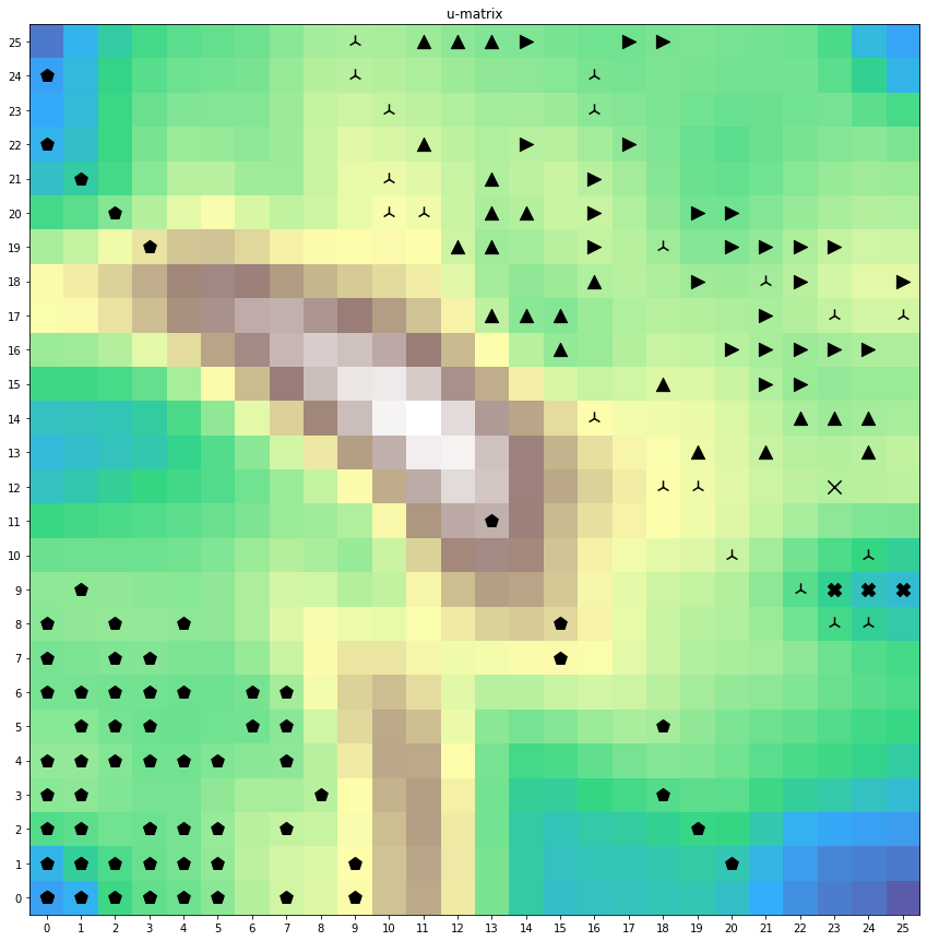
An example of a trained SOM using musical pieces of Kachin ethnic group, northern Myanmar with Uyghur musical pieces from Xinjiang, western China is shown below. The map is trained with 5-grams. Most Uyghur pieces are located at the lower blue region, mainly because of the frequent tone repetitions of Uyghur music compared to Kachin songs.

Trained 5-gram SOM, comparing Kachin and Uyghur musical pieces. Most Uyghur pieces are located in the lower blue region due to enhanced note repetition found in Uyghur music.
Tonal System
Tonal systems are normally understood as a small set of cent values. So a 7-tone scale has seven-pitch values. Still, depending on musical performance, determining a tonal system is more or less complex. Articulation in singing often leads to a large variation in pitch. The same might hold for lutes, guitars, violins, or wind instruments. Percussion instruments have a much more straight pitch. till, they often are inharmonic, and, therefore, a pitch might not even be perceived.
Therefore the MIR tool for investigating tonal systems takes tonal systems as an accumulation of pitch values over mainly single-voiced musical pieces compressed within one octave with a precision of one cent. An autocorrelation algorithm determines the pitch for n time frames per second, the one already shown in the melody section above.
In a second stage, pitch events are detected, again as discussed above. All pitches of the detected musical events are then accumulated in dcent values (dcent = 1 is recommended), starting again from f0 in noctaves. To also include melismas and slurs in the calculation, the tonal system is derived from all pitch values in the musical event (top left plot of above figure). If the tonal system should only be constructed from pitch events with a very constant pitch, the mindev parameter needs to be small.
The strongest frequency maxf is then taken as the fundamental of the tonal system. In the tonal system plots shown below, this lowest cent is not shown, as it often overwhelms the other accumulated cent values.
In a last step, using the largest accumulated pitch as fundamental of the tonal system, all accumulated cents in noctaves are mirrored into one octave. When a precision of one cent was used, the input feature vector to the SOM has a length of 1200, reflecting 1200 cent in one octave.
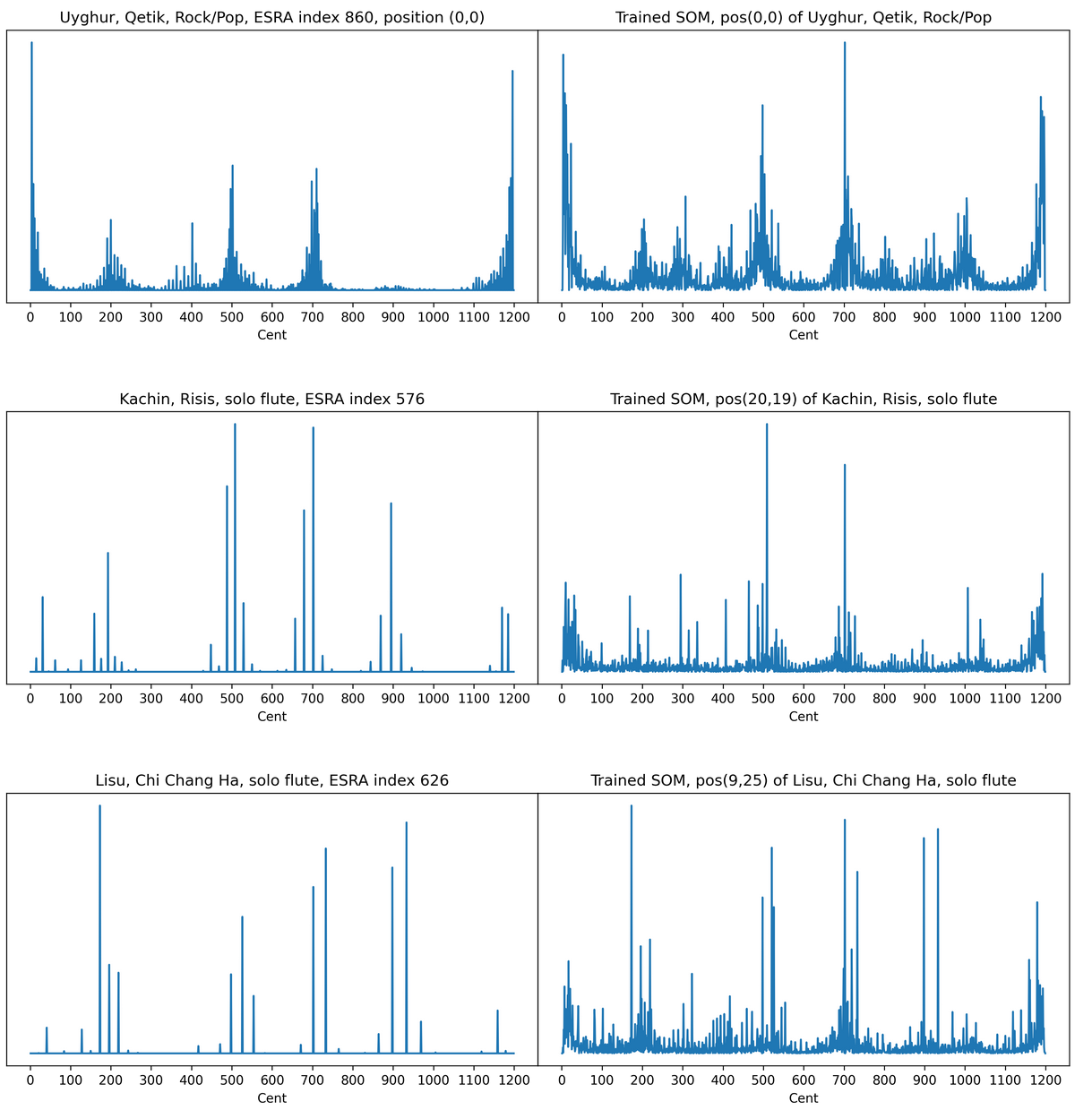
Three examples of tonal systems as calculated from a sound file (left column) and as a vector on the neural map on the location the musical pieces fits best (right column). Top: Uygur Rock/Pop piece by Qetik, Middel: Kachin flute solo piece, Bottom: Lisu flute solo piece.
The outputs are
accumulated cent values over noctaves
accumulated cent values within one octave
Names of the ten best-matchin tonal systems
Cent values of the best-matching tonal systems
Correlation of each cent value in all best-matching scale to estimate the salience of each note to the overall large correlation between theoretical scale and calculated values
Overall correlation of the best-matching scales
The tonal systems used for comparison are taken from a set of scales: https://www.flutopedia.com/scales.htm. The list contains over 900 scales. Therefore, matches might not meet expectations. Reduced lists fitting special intrests will be developed in the future.
Below, a trained SOM with tonal systems of the Kachin vs. Uyghur music case is shown below. Both ethnic groups are clustered, where Uyghur pieces on the lower left are nearer to just intonation, while Kachin shows more deviating pitches.
Rhythm Track
ESRA includes musical pieces from more than 70 ehtnic groups collected in over 50 countries. A reasonable system for rhythm similairity estimation has to
The rhythm track implemets a timbre-based theory of musical rhythm Blaß [Blass13] [Blaß2019]). That means, it does not address the relative temporal distance between note onsets. Instead it focuses on the actual sounds that are played. To this end, ESRA runs an onset detection algorithm, which estimates the temporal position of note onsets within the piece under consideration. Thereafter, audio features extraction computes a measure for the perceived brightness of the sounds at each onset. ESRA then estimates the probabilites to change from one given sound to another. This analysis is carried out using a Hidden Markov Model.
This approch to rhythm has several advantages:
Since the model operates only on the actual sound, it avoids any cultural bias. Especially, the model does not apply notions of Western rhythm theories to other music cultures.
The numerical representatin of the rhythm is of exactly the same size for each piece analyzed in the same track no matter how long the actual piece is. This is a crucial feature for further processing stages.
Musical from literally any music culture a be compoared on a well-defined basis.
However, the model does have a some disadvantages, too. These include first, that temporal information is reduced to a equidistant succession. Additionally, the model as such can be “hard to read” for humans. This fact is, however, mitigated by system structure. Since the models are automatically compared, users only have to interprete the ouput of the similarity estimation, which is straight foreward. They, hence, do not have to care too much about details of the rhythm model.
Onset detection
Onset detection estimates the starting points of note onsets in digital audio signals. Our approach is based on the standard spectral flux method. An onset is assumed between two consecutive STFT segements if there is a high per band difference in spectral energy.
Further details can be found in the documentation of the spectral_flux() method and the FluxOnsetDetector class from the apollon framework.
Audio feature extraction
ESRA descrbies the timbre of an onset in terms of the perceived brightness. The spectral centroid is know to correlated well with the perception of brightness.
Timbre Track
The TimbreTrack combines a set of audio features to model the timbral content of piece of music. These features are computed on short, consecutive portions of the input signal.
Frequency domain features
Frequency domain features are computed from a spectrogram. A spectrogram displays the distribution of energy within the audible frequency bands of consecutive, short portions of the input signal. ESRA computes its spectrograms using the Discrete Fourier Transform.
The shape of each spectral distributions is related to how humans perceive the timbre of the related portion of a musical piece. Typically, the first four moments of a distribution are utilized to describe its shape.
Spectral Centroid
The first moment of a spectral energy distribution is the spectral centroid frequency. It is a measure of central tendency. It marks the frequency that is considered as the center of a spectrum. It may be computed as the weighted arithetic mean of a frequency spectrum.
Several studies could confirm that the spectral centroid correlates strongly with the human auditory perception of brightness. Moreover, brightness is the most salient dimension of timbre perception.
Detailed information can be found in apollon.signal.features.spectral_centroid.
Spectral Spread
Spectral Spread is the second moment of a spectral distribution and refers to its variance. It is a measure of how much frequencies deviate from the spectral centroid frequency.
Unlike Spectral Centroid, Spectral Spread does not map immediately to a perceptional quality.
Detailed information can be found in apollon.signal.features.spectral_spread.
Spectral Skewness
Spectral skewness is the third spectral moment. A skewness of 0 means that the distribution is perfectly symmetric. Negative values indicate a bias towards high frequency. Conversely, positive values indicate a displacement to low frequencies.
Detailed information can be found in apollon.signal.features.spectral_skewness.
Spectral Kurtosis
Spectral kurtosis is the fourth spectral moment. It is a measure for the shape of the tails of a distribution.
Detailed information can be found in apollon.signal.features.spectral_kurtosis.
Spectral Flux
Spectral flux is the change in amplitude per frequency bin over time. It is particularly useful for timbre.
Detailed information can be found in apollon.signal.features.spectral_flux.
Time domain features
Fractal correlation dimension
The fractal correlation dimensions measures chaoticity. Chaoticity is defined the the amount of harmonic overtone spectra plus large amplitude fluctuations. So a single guitar tone in its steady-state has a fractal correlation dimension of one. A piano chord with three keys pressed has a fractal dimension of three. Each inharmonic sinusoidal added another dimension. White noise therefore has a dimension of infinity.
To calculate a fractal correlation dimension, a time series x(t) of recorded sound with n sample points is embedded in a pseudo phase-plot like
Starting from X(t) we then calculate the ‘area’ or ‘volume’ C(r) like
Here, H(x) is the Heavyside function with
which counts the amount of points within the radius r. C(r) is a probability, as we normalize with respect to all \(N^2\) possible combinations.
Then the correlation dimension is defined as
which is derived from the idea of the definition of the dimension (Bader2013). The exponent is the dimension which is the slope of a log-log plot. So practically we need to take the middle of the distribution and look for a constant slope in the log-log plot. This slope is the correlation dimension.
This is a very powerful tool as it has certain properties:
If only one harmonic overtone spectrum is in the sound, DC = 1 no matter how many overtones are present.
Each additional harmonic overtone spectrum raises DC to the next integer.
If only one inharmonic sinusodial is added, DC raises to the next integer making it suitable for detection of additional single inharmonic components too.
Large amplitude fluctuations lead to a raise of DC.
As the absolute amplitude is normalized, DC does not depend upon amplitude.
If a component is below a certain amplitude threshold it is no longer considered by the algorithm.
The fractal correlation dimension raises with initial transients, as they contain chaoticity. It is also a good measure of event density in a musical piece.
Models of perceptional qualities
Loudness
Although several algorithms of sound loudness have been proposed by Fastl and Zwicker [FZ07], for music still no satisfying results have been obtained [vR13]. Most loudness algorithms aim for industrial noise and it appears that musical content considerably contributes to perceived loudness. Also loudness is found to statistically significantly differ between male and female subjects due to the different constructions of the outer ears between the sexes. Therefore a very simple estimation of loudness is used, and further investigations in the subject are needed. The algorithm used is
This corresponds to the definition of decibel, using a rough logarithm-of-ten compression according to perception, and a multiplication with 20 to arrive at 120 dB for a sound pressure level of about 1 Pa. Of course the digital audio data are not physical sound pressure levels (SPL), still the algorithm is used to obtain dB-values most readers are used to. As all psychoacoustic parameters are normalized before inputting them into the SOM, the absolute value is not relevant.
Roughness
Roughness calculations have been suggested in several ways (for a review see [SvRB09] and [Bad13]). Basically two algorithms exist, calculating beating of two sinusoidals close to each other [SvRB09, Set93, vH63] or integrating energy in critical bands on the cochlear [FZ07, Sot94]. The former has been found to work very well with musical sounds, the latter with industrial noise.
In the paper a modified Helmholt/Bader algorithm is used. Like Helmholtz it assumes a maximum roughness of two sinusoidals at 33 Hz frequency difference. As Helmholtz did not give a mathematical formula how he did calculate roughness, according to his verbal descriptions a curve of the amount of roughness \(R_n\) is assumed between two frequencies with distance \(df_n\) which have amplitudes \(A_1\) and \(A_2\) like
with a maximum roughness at \(f_r=33\) Hz. The roughness \(R\) is then calculated as the sum of all possible sinusoidal combinatins like
The goal of Schneider et al. [SvRB09] was to model the perceptual differences of tuning systems like Pure Tone, Werkmeister, Kirnberger, etc. in a Baroque piece of J. S. Bach. This task required high temporal and spatial resolution in the frequecy domain. The authors, therefore, utilized a Discrete Wavelet Transform (DWT). The roughness analysis in ESRA does not aim for such subtle differences, but for an overall estimation. Moreover, ESRA has to accomodate resource restrictions. To this end, the DWT was replaced by the Discrete Fourier Transform.
Sharpness
Perceptual sharpness is related to the work of Bismarck (Bismarck1974) and followers (Aures1985b, Fastl2007). It corresponds to small frequency-band energy. According to (Fastl2007) it is measured in acum, where 1 acum is a small-band noise within one critical band around 1 kHz at 60 dB loudness level.
Sharpness increases with frequency in a nonlinear way. If a small-band noise increases its center frequency from about 200 Hz to 3 kHz, sharpness increases slightly, but above 3 kHz strongly, according to perception that very high small-band sounds have strong sharpness. Still sharpness is mostly independent of overall loudness, spectral centroid, or roughness, and therefore qualifies as a parameter on its own.
To calculate sharpness the spectrum A is integrated with respect to 24 critical or Bark bands, as we are considering small-band noise. With loudness \(L_B\) at each Bark band \(B\), sharpness is
where a weighting function $g_B$ is used strengthening sharpness above 3 kHz like({Peeters2004}
Example
Below the an example result of two sets of Hip Hop musical pieces. A SOM was trained with a certain amount of features, able to cluster Chinese (red) and Western (violet) Hip Hop pieces.
